Melting ice cream and chocolate bunny

Disclaimer: This method for “melting ice cream and chocolate bunnies” is not my creative idea. I was inspired by the article Melting and Flowing by Mark Carlson, Peter J. Mucha, R. Brooks Van Horn III, Greg Turk, and others. And all the contents below comes from my understanding of this paper. The ice cream bunny is also shown in the original article, while the chocolate bunny is my own creation.

Melting Ice cream Bunny:

FRONT		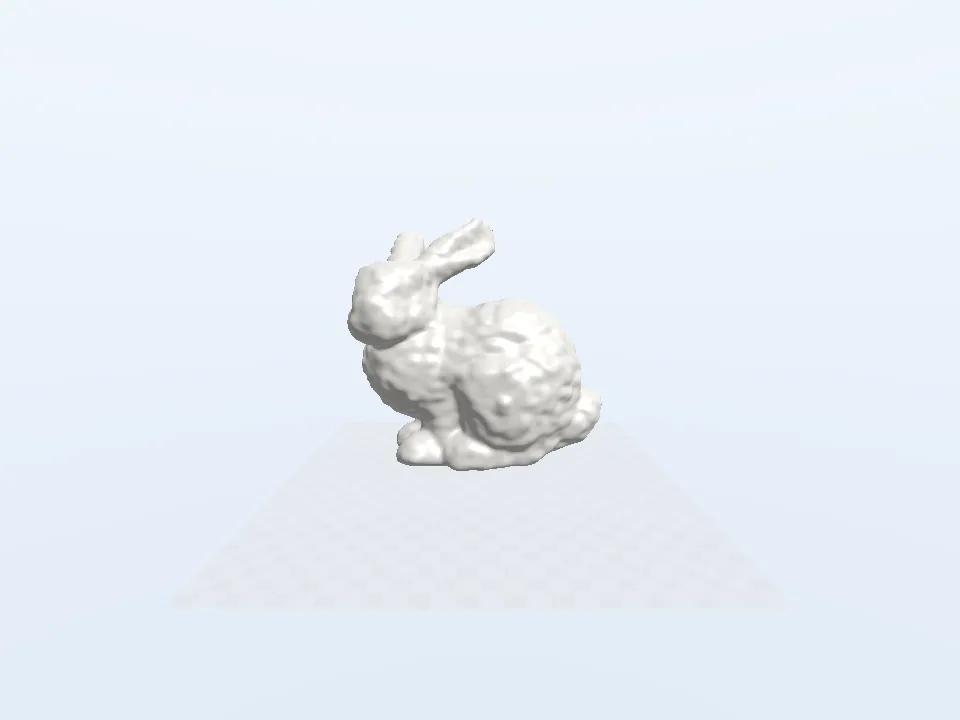	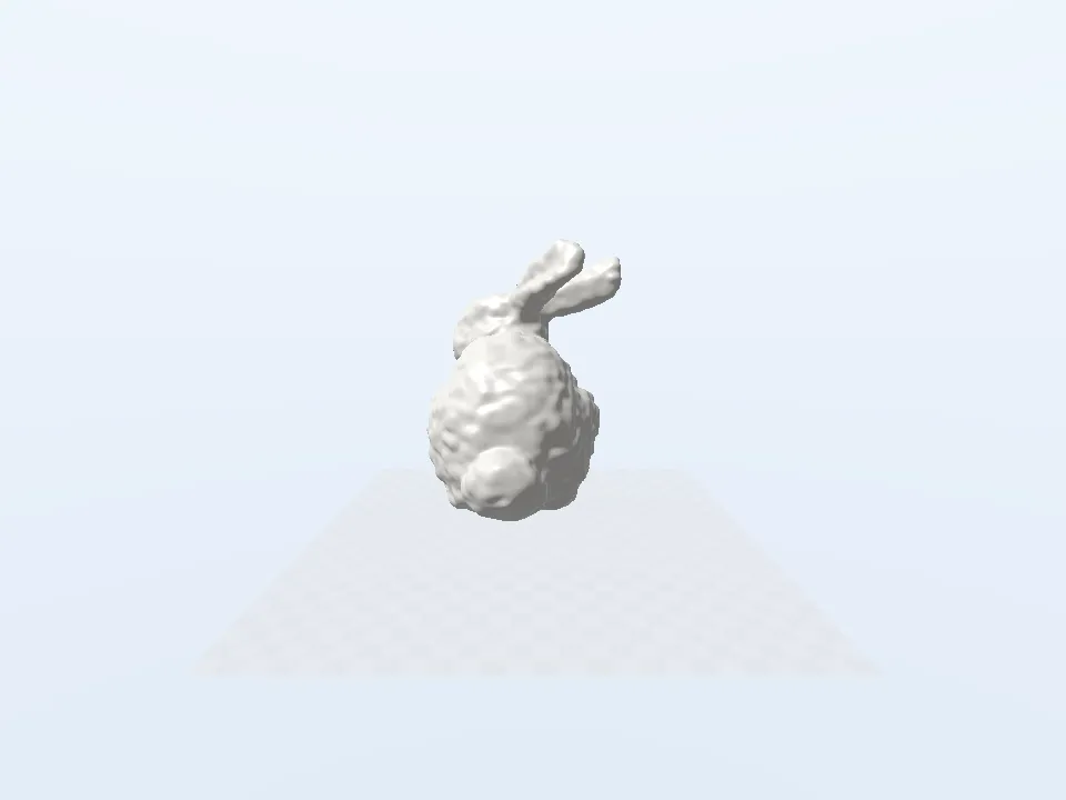SIDE
TOP		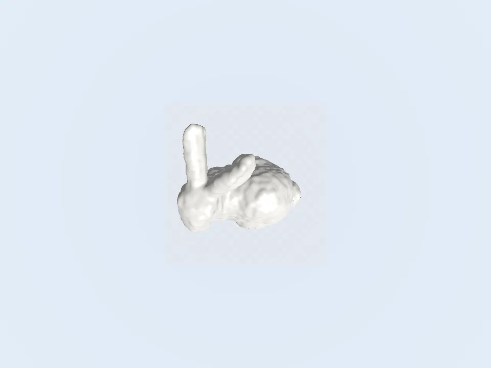	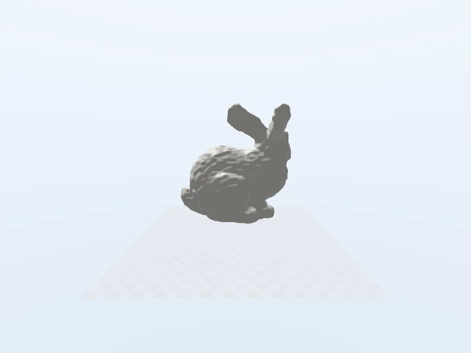BACK

Melting chocolate Bunny:

FRONT		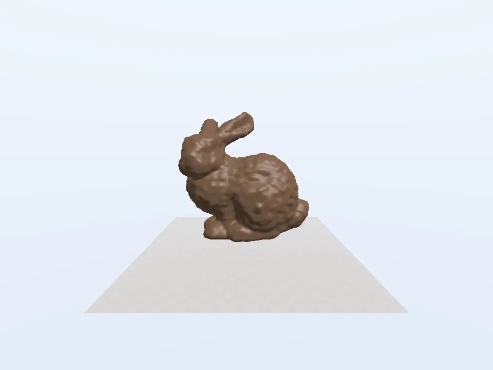	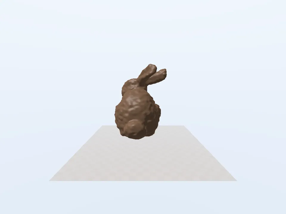SIDE
TOP		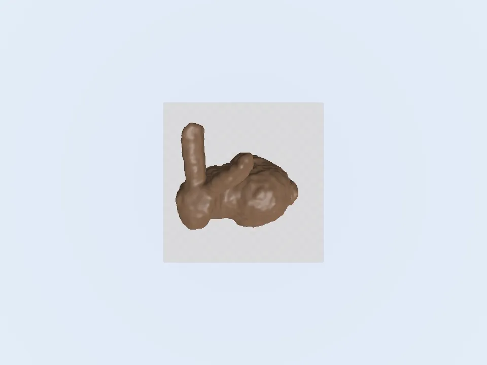	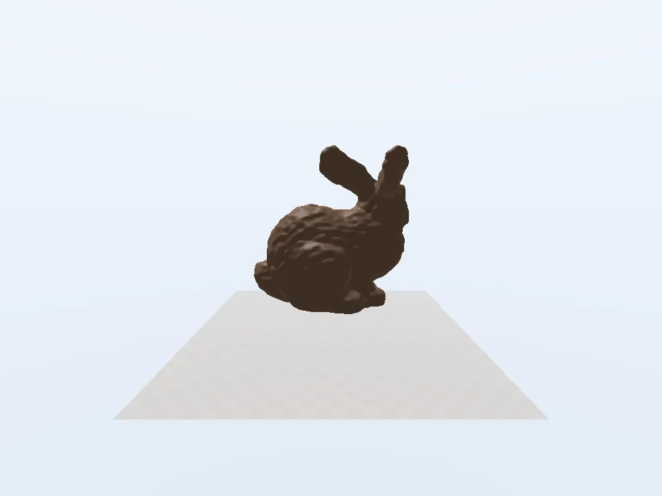BACK

The source cuda code can be found here: melting ice cream bunny and melting chocolate bunny, which you should noted is that the stb_image.h, stb_image_write.h and the stanford-bunny.obj must be placed at the same file level.

1. Overview

The goal is to use one unified fluid framework to cover a continuous transition: “near-solid -> semi-fluid -> low-viscosity liquid”.

Core strategy:

Use incompressible viscous flow equations for motion.
Use a temperature field to drive viscosity changes.
Use implicit diffusion for high-viscosity stability.
Use particles to mark free surfaces and reconstruct renderable geometry.

2. Governing Equations

2.1 Incompressibility Constraint

\nabla \cdot u = 0

2.2 Momentum Equation (Variable Viscosity)

\frac{\partial u}{\partial t} = - (u \cdot \nabla) u + \nabla (ν \nabla u) - \frac{1}{ρ} \nabla p + f

Where:

$u$ : velocity field
$ν$ : kinematic viscosity (space/time varying)
$p$ : pressure
$f$ : body force (usually gravity)

2.3 Temperature Transport Equation

\frac{\partial T}{\partial t} = k \nabla^{2} T - (u \cdot \nabla) T + Q

$T$ : temperature
$k$ : thermal diffusivity
$Q$ : heat source/cooling term

3. State Representation (Eulerian + Lagrangian)

The method uses a hybrid representation:

Eulerian grid: stores velocity, pressure, temperature, viscosity, fluid flags.
Lagrangian particles: track the free surface, avoiding coarse-grid-only artifacts.

At the end of each step, particles write back which cells are fluid.

4. Time Integration (Operator Splitting)

Each time step is split into:

Advection + body force (explicit)
Viscous diffusion (implicit)
Pressure projection (enforce incompressibility)
Particle advection + fluid marker rebuild
Temperature advection + temperature diffusion + heating/cooling
Viscosity update from temperature

Equation form:

4.1 Advection + Body Force

u^{*} = u^{n} + Δ t [- (u \cdot \nabla) u + f]

4.2 Implicit Viscous Diffusion

u^{**} = u^{*} + Δ t \nabla (ν \nabla u^{**})

Discrete linear system:

(I - Δ t L_{ν}) u^{**} = u^{*}

4.3 Pressure Projection

Solve Poisson first:

\nabla^{2} p = \frac{ρ}{Δ t} \nabla \cdot u^{**}

Then correct velocity:

u^{n + 1} = u^{**} - \frac{Δ t}{ρ} \nabla p

5. Variable-Viscosity Discretization and Face Viscosity

With variable viscosity, diffusion is no longer a constant-coefficient Laplacian.
Viscosity should be defined at cell faces, e.g.:

ν_{i + 1/2, j, k}

A practical face viscosity is the geometric mean:

ν_{f a ce} = ν_{L} ν_{R}

Compared to arithmetic averaging, this often reduces over-damping when melt drips flow along high-viscosity regions.

6. High-Viscosity Stability and Implicit Solving

Explicit diffusion has a strict stability condition:

ν Δ t / h^{2} < O (1)

For high viscosity, $Δ t$ becomes prohibitively small.
So diffusion should be implicit, solved iteratively (CG/Jacobi/PCG, etc.).

Desirable system properties:

Symmetric
Positive definite
Sparse

These properties improve solver robustness and efficiency.

7. Free-Flight Momentum Reintroduction

At high viscosity, implicit diffusion can artificially kill velocity of detached flying blobs.
A practical correction:

Identify connected fluid components not touching solid boundaries.
Compute pre-/post-diffusion bulk velocity:

v_{b u l k}^{p re}, v_{b u l k}^{p os t}

Add the difference back to all cells in that component:

Δ v = v_{b u l k}^{p re} - v_{b u l k}^{p os t}

u \leftarrow u + Δ v

This mostly restores translational momentum, which is usually enough to prevent the “frozen-in-air” artifact.

8. Temperature Solve and Heat Source Model

8.1 Temperature Advection

T^{*} = T^{n} - Δ t (u \cdot \nabla T)

8.2 Implicit Temperature Diffusion

(I - Δ t k \nabla^{2}) T^{n + 1} = T^{*} + Δ t Q

8.3 Practical Heating/Cooling Terms

Common engineering choices:

Ambient cooling: $Q_{coo l} \propto (T_{e n v} - T)$
Local heater: distance-weighted heat injection

Q_{h e a t er} \propto w (r) (T_{h e a t er} - T), w (r) = max (0, 1 - r / R)

9. Temperature-to-Viscosity Constitutive Mapping

Melting requires viscosity to span multiple orders of magnitude.
A practical mapping:

Normalize temperature into a melt transition band: $s \in [0, 1]$
Use a smooth function (e.g., smoothstep) to avoid hard jumps
Interpolate viscosity in log-space

s = smoothstep (T_{m} - Δ T, T_{m} + Δ T, T)

ν (T) = exp ((1 - s) ln ν_{co l d} + s ln ν_{h o t})

This gives “near-solid at low temperature, rapid liquefaction near melt”.

10. Free-Surface Reconstruction (Particle Splatting)

Renderable surfaces are usually not extracted from the coarse simulation grid directly:

Build a higher-resolution volume $V$
Splat surface particles into volume (tent kernel)

V (x) + = a \in {x, y, z} \prod max (0, 1 - \frac{∣ a - a _{p} ∣}{r})

Clamp + low-pass smoothing
Iso-surface extraction (or direct volume ray marching)

A typical practical kernel width is around 2.5 voxels.

11. Minimal End-to-End Pipeline

Initialize: OBJ voxelization + particle seeding.
Main loop: coupled velocity/pressure/temperature/viscosity updates.
Advect particles and rebuild fluid markers.
Splat particles into high-res volume.
Render and export frame sequence.

12. Parameter Tuning Guide (Bunny Melting)

Tune three groups first:

Viscosity range: $ν_{co l d}, ν_{h o t}$
Melt center and transition width: $T_{m}, Δ T$
Heat input strength/range: $T_{h e a t er}, R, gain$

Practical effects:

More “solid feel”: increase $ν_{co l d}$ , decrease $Δ T$ .
More “runny melt”: decrease $ν_{h o t}$ , increase heater radius or gain.
Less numerical jitter: increase implicit iterations or reduce substep size.

13. Validation Criteria

A good melting simulation should satisfy:

Local melting starts first (not globally uniform softening).
High-viscosity and low-viscosity regions coexist in the same frame.
Detached droplets keep inertia and do not instantly stall from diffusion.

If these three are met, the melting-method chain is usually correct.